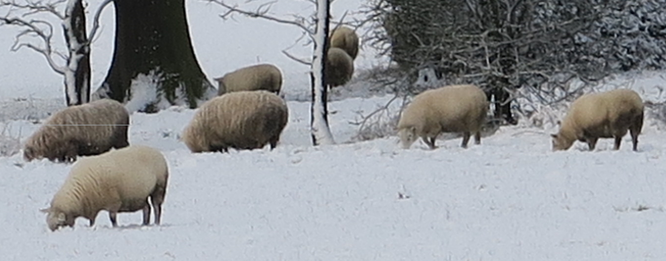
This model describes radiocaesium transfer in the lovely sheep shown below. They are busy trying to get to the grass beneath the snow, not at all bothered by a little bit of radioactivity!

A number of interconnected  ‘pools’ of radiocaesium (the boxes in the diagram) are considered, with transfers of radiocaesium occurring between the pools (the arrows).

Mathematically each radiocaesium pool is represented by a differential equation with the transfers between pools (the arrows) given by a constant coefficient multiplied by the tissue value. As an example the equation for muscle (M) is

   

The rate at which radiocaesium enters the muscle from the extra cellular fluid (ECF) is given by the value of ECF multiplied by the rate coefficient a_em. Similarly the rate at which radiocaesium leaves the muscle is the value of M multiplied by the rate coefficient a_me. The choice of symbols (i.e. notation) is a matter of preference, but in this case all the rate coefficients use ‘a’ with a subscript to denote the source and destination of the transferred radiocaesium (e.g. a_me for muscle to extra cellular fluid).

The overall model comprises a series of equations all very similar to the one shown for muscle. The equation for extra cellular fluid (ECF) has a lot more terms, because it is the main exchange pool in the system. This sort of model is very easily set up in OpenModel using ODEs for the tissue differential equations and parameters for the rate coefficients.

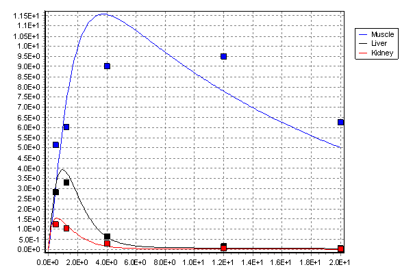
In the published model the values of the rate coefficients were estimated by fitting the model to a set of observations. An example of the resulting fit is shown below for three important tissues, muscle, kidney and liver (the main tissues used for food in UK animal production systems).

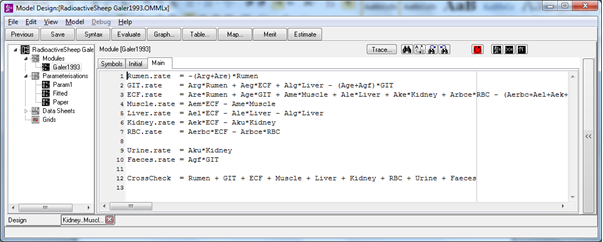
Implementing this model and fitting is very straightforward in OpenModel; it is exactly the sort of application for which OpenModel was intended. Key practical issues that arise are setting up the equations, maintaining different sets of potential rate coefficient values, using the deviation of observations from model predicted values to fit the model, and controlling how the deviation is calculated. OpenModel provides the means to manage all these aspects of model development.

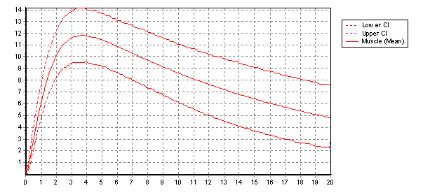
Follow up considerations are typically estimation of confidence intervals on predictions (as shown below)and investigating choices about model design (i.e. is there a better set of equations to do the job?). Again OpenModel supports these very practical aspects of model development.

The model is fully described by Galer et al (1993) and more details of the OpenModel implementation are given in the Example Applications guide in the OpenModel download. As it happens the biology of the model was later revised by Crout at el (1996). The arrangement of the tissues was made more realistic and concentrations used as state variables rather than total radiocaesium. Of course, both versions of the model are now rather old but nevertheless make good examples for the use of model fitting in OpenModel.

References

Crout NMJ, Beresford NA, Howard BJ, Mayes RW, Assimakopoulos PA, Vandecasteele C. (1996). The development and testing of a revised model of radiocaesium transfer to sheep tissues. Radiation & Environmental Biophysics 35:19-24

Galer AM, Crout NMJ, Beresford NA, Howard BJ, Mayes RW, Barnett CL, Eayres H, Lamb CS (1993). Dynamic radiocaesium distribution in sheep: measurement and modelling. J. Environ. Rad. 20:35-48.